Digital Materials Science

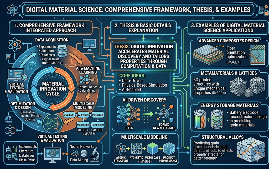
Digital Materials Science is the application of computational methods, data-driven techniques, artificial intelligence, and digital simulation tools to understand, design, predict, and discover new materials — accelerating discovery cycles from decades to years, or even months.

Traditional materials science relied on trial-and-error experimentation. Digital Materials Science replaces or supplements this with virtual experimentation, predictive modeling, and high-throughput screening, enabling researchers to explore vast compositional and structural spaces that would be physically or economically impossible to test experimentally.

Foundational Statement: “The future of materials development lies not in the lab alone, but in the synergy between physical experiments and digital intelligence — where atoms are modeled before they are synthesized.”

Using physics-based mathematical models to simulate how atoms, molecules, and macroscopic structures behave under various conditions — without physical samples.

Density Functional Theory (DFT)

Quantum mechanical simulation of electron behavior in atoms and molecules.

Predicts: electronic structure, bonding energy, lattice constants, bandgaps, magnetic properties.

Software: VASP, Quantum ESPRESSO, CASTEP.

Example: Predicting the electronic bandgap of a new perovskite solar cell material before synthesis.

B. Molecular Dynamics (MD)

Simulates atomic motion over time using Newton’s equations of motion.

Predicts: thermal conductivity, diffusion, mechanical deformation, phase transitions.

Scale: Nanometers, nanoseconds.

Software: LAMMPS, GROMACS, NAMD.

Example: Simulating how lithium ions diffuse through a solid electrolyte in a battery — identifying bottlenecks before building a prototype.

C. Monte Carlo (MC) Simulation

Uses random sampling to explore statistical mechanical behavior of materials.

Predicts: equilibrium properties, phase diagrams, ordering phenomena.

Software: MCMD, custom Python scripts.

Example: Exploring how temperature affects atomic ordering in a cobalt-iron alloy.

D. Phase-Field Modeling

Mesoscale method simulating microstructure evolution (grain growth, solidification, crack propagation).

Scale: Micrometers, milliseconds.

Software: MOOSE, OpenPhase.

Example: Simulating grain growth in a steel alloy during heat treatment to optimize hardness.

E. Finite Element Analysis (FEA)

acroscale simulation of mechanical, thermal, and electrical behavior of components.

Scale: Component to structural level.

Software: ANSYS, Abaqus, COMSOL.

Example: Predicting stress distribution in a turbine blade under high temperature — guiding alloy selection.

PILLAR 2: Data-Driven Discovery (AI/ML in Materials)

What it is: Using machine learning and artificial intelligence to identify patterns in materials data, predict properties of unsynthe­sized compounds, and guide experimental discovery.

Key Methods:

A. Machine Learning Potentials (MLPs)

Neural networks trained on DFT data to replicate quantum accuracy at MD speeds.

1,000–1,000,000x faster than DFT.

Types: Behler-Parrinello NN, Graph Neural Network potentials (GNNs), MACE, NequIP.

Example: Training a GNN on 100,000 DFT calculations of metal oxides, then using it to screen 10 million compositions for battery cathode candidates in days.

B. Property Prediction Models

Supervised ML models trained on experimental or DFT databases to predict target properties.

Inputs: composition, crystal structure, processing conditions.

Outputs: hardness, conductivity, melting point, corrosion resistance, etc.

Algorithms: Random Forest, XGBoost, Graph Convolutional Networks (GCN).

Example: Predicting the Curie temperature of magnetic alloys from composition alone, reducing experimental screening by 90%.

C. Generative AI for Materials Design

Generative models propose entirely new crystal structures or molecules with desired properties.

Methods: Variational Autoencoders (VAE), Generative Adversarial Networks (GAN), Diffusion Models, Large Language Models.

Example: DiffCSP (a diffusion model) generates crystal structures conditioned on a target bandgap — outputting candidate structures for photovoltaics that have never existed before.

D. Natural Language Processing (NLP) for Literature Mining

AI reads millions of scientific papers to extract materials data automatically.

Tools: MatBERT, ChemDataExtractor, GPT-based extractors.

Example: Automatically extracting synthesis conditions and reported properties from 2 million materials science papers to build a training dataset.

E. Databases Enabling AI

Materials Project: 150,000+ computed material properties (DFT-based).

AFLOW: 3.5 million+ materials data entries.

OQMD (Open Quantum Materials Database): thermodynamic data.

COD (Crystallography Open Database): experimental crystal structures.

These databases serve as training sets for ML models and as search spaces for high-throughput screening.

Digital Twins for Materials

What it is: A digital twin is a real-time, dynamic virtual replica of a physical material or component that continuously updates based on sensor data from the real world — enabling predictive maintenance, performance optimization, and failure prediction.

Components:

Physical asset (material/component/structure)

Sensor network (temperature, strain, corrosion, vibration)

Digital model (physics simulation + ML surrogate)

Data integration layer (real-time synchronization)

Decision/optimization engine

Example 1 — Aerospace: A turbine blade in a jet engine has a digital twin that receives live temperature and stress data from embedded sensors. The twin updates its fatigue model in real time, predicting exactly when microcracking will initiate — scheduling maintenance before failure, not on fixed schedules.

Example 2 — Battery Systems: A lithium-ion battery pack in an electric vehicle has a digital twin that tracks degradation of electrode materials at the particle level, predicting remaining useful life and optimizing charging protocols to extend battery life.

Example 3 — Civil Infrastructure: A concrete bridge has a digital twin incorporating corrosion models for the rebar and fracture mechanics for the concrete — ingesting data from humidity sensors, strain gauges, and periodic NDT scans.

PILLAR 4: High-Throughput Computational Screening

What it is: Automated, parallelized computational workflows that evaluate thousands to millions of candidate materials in silico — narrowing the search space before any physical experiment is done.

Workflow:

Define target property (e.g., thermoelectric efficiency, hydrogen storage capacity)

Define compositional search space (e.g., all ternary oxides)

Automated DFT/ML calculations on HPC clusters

Filter by thermodynamic stability, synthesizability, toxicity

Rank candidates → forward to experimental validation

Tools:

Pymatgen: Python library for materials analysis and structure manipulation.

ASE (Atomic Simulation Environment): Interface for running and analyzing simulations.

FireWorks, AiiDA: Workflow management for HPC environments.

Atomate: Automated DFT workflows built on Pymatgen + FireWorks.

Example: The Materials Genome Initiative (USA) used high-throughput DFT to screen 68,000 candidate solid-state electrolytes for lithium batteries in a single computational campaign — identifying 21 promising candidates that were then synthesized and tested experimentally.

What it is: Closed-loop systems where digital predictions guide experiments, and experimental results feed back into computational models — creating an accelerating cycle of discovery. Also called the “self-driving laboratory” or “autonomous materials discovery.”

The Closed-Loop Cycle:

Digital model proposes candidates

Robotic synthesis platform synthesizes candidates

Automated characterization (XRD, SEM, spectroscopy)

Data fed back to AI/model

Model refines predictions → repeat

Example — Self-Driving Labs: The Accelerated Innovation for the Autonomous Generation of Experiments (A-Lab) at Lawrence Berkeley National Lab uses robotic synthesis, automated powder XRD, and a Bayesian optimization AI to discover new inorganic solid-state materials with zero human intervention between cycles.

Example — Combinatorial Libraries: Thin-film deposition systems create composition gradient libraries (thousands of slightly different alloy compositions on a single wafer). Automated profilometry and conductivity mapping scan all compositions simultaneously — paired with ML analysis to identify the optimal composition for a target property.

CROSS-CUTTING THEMES

A. The Materials Genome Initiative (MGI) Philosophy Launched in 2011 by the US government, the MGI established the framework of integrating experiment, computation, and databases to halve the time and cost of discovering and deploying new materials. It is the intellectual foundation of modern Digital Materials Science.

B. Multi-Scale Modeling No single simulation method spans all relevant length and time scales. Digital Materials Science requires seamless handoff of information between scales:

• Quantum (DFT) → Atomistic (MD) → Mesoscale (phase-field) → Macroscale (FEA)
• This is called concurrent or hierarchical multiscale modeling.
• Example: Crack propagation in a metal: DFT gives crack-tip bond energies → MD simulates dislocation dynamics → phase-field grows the crack → FEA predicts structural failure.

C. Uncertainty Quantification (UQ) Every digital prediction carries uncertainty. Rigorous digital materials science includes:

• Propagating model uncertainty through predictions.
• Knowing when to trust the model vs. when to run an experiment.
• Bayesian methods are dominant here — they naturally quantify confidence.

D. FAIR Data Principles Findable, Accessible, Interoperable, Reusable data is a prerequisite for AI-driven materials science. Siloed, poorly-formatted experimental data cannot feed ML models. The field is building shared ontologies (e.g., EMMO — Elementary Multiperspective Materials Ontology) to standardize materials data globally.

APPLICATIONS WITH EXAMPLES

Domain	Challenge	Digital Approach	Result
Energy Storage	Find better lithium battery cathodes	HT-DFT + ML screening	LiNiMnCoO2 variants optimized for energy density
Solar Energy	Maximize perovskite solar cell efficiency	DFT bandgap prediction + composition optimization	Identified mixed halide perovskites exceeding 25% efficiency
Structural Alloys	Design lightweight, high-strength steels	CALPHAD + phase-field + ML	Reduced alloy development from 10 years to 2 years
Semiconductors	Discover topological insulators	DFT + symmetry analysis	1000+ candidate topological materials identified computationally
Hydrogen Storage	Screen metal-organic frameworks (MOFs)	ML on MOF databases	Identified high-capacity hydrogen adsorbents for fuel cells
Drug Delivery	Design biocompatible polymer nanocarriers	MD simulation + ML	Optimized polymer architecture for drug release kinetics
Corrosion Protection	Predict coating failure	Digital twin + sensor fusion	40% reduction in unplanned maintenance in oil pipelines

CHALLENGES & FUTURE DIRECTIONS

Current Challenges:

Accuracy-cost tradeoff — DFT is accurate but slow; ML is fast but needs data.

Synthesizability gap — computationally stable structures may be experimentally impossible to make.

Data scarcity — ML needs large, clean datasets; much experimental data is unpublished or inconsistent.

Property extrapolation — models trained on known materials struggle to generalize to truly novel compositions.

Integration — connecting simulation tools across scales remains technically complex.

SUMMARY

Digital Materials Science represents a paradigm shift from empirical, slow, resource-intensive materials development to a data-rich, simulation-driven, AI-augmented discipline. Its core thesis is that the properties of matter are ultimately governed by physics that can be captured in equations, and that equations can be solved computationally — meaning the right material for any application can, in principle, be found without ever touching a test tube first.

The framework integrates five pillars: physics-based simulation (from quantum to macroscale), machine learning for pattern extraction and property prediction, digital twins for real-time monitoring and prognosis, high-throughput computational screening for broad compositional exploration, and closed-loop autonomous workflows where robots and AI replace manual experimental cycles. Together these pillars compress the historical 20-year timeline from materials discovery to deployment toward a target of 2–5 years.

The discipline’s full realization depends on solving three bottlenecks: data quality and availability, model transferability beyond training distributions, and seamless multiscale integration. As these are solved — partly through foundation models, partly through global database standardization, and partly through hardware advances in quantum computing — Digital Materials Science is positioned to underpin the next generation of energy storage, structural engineering, semiconductors, and biomedical devices.