
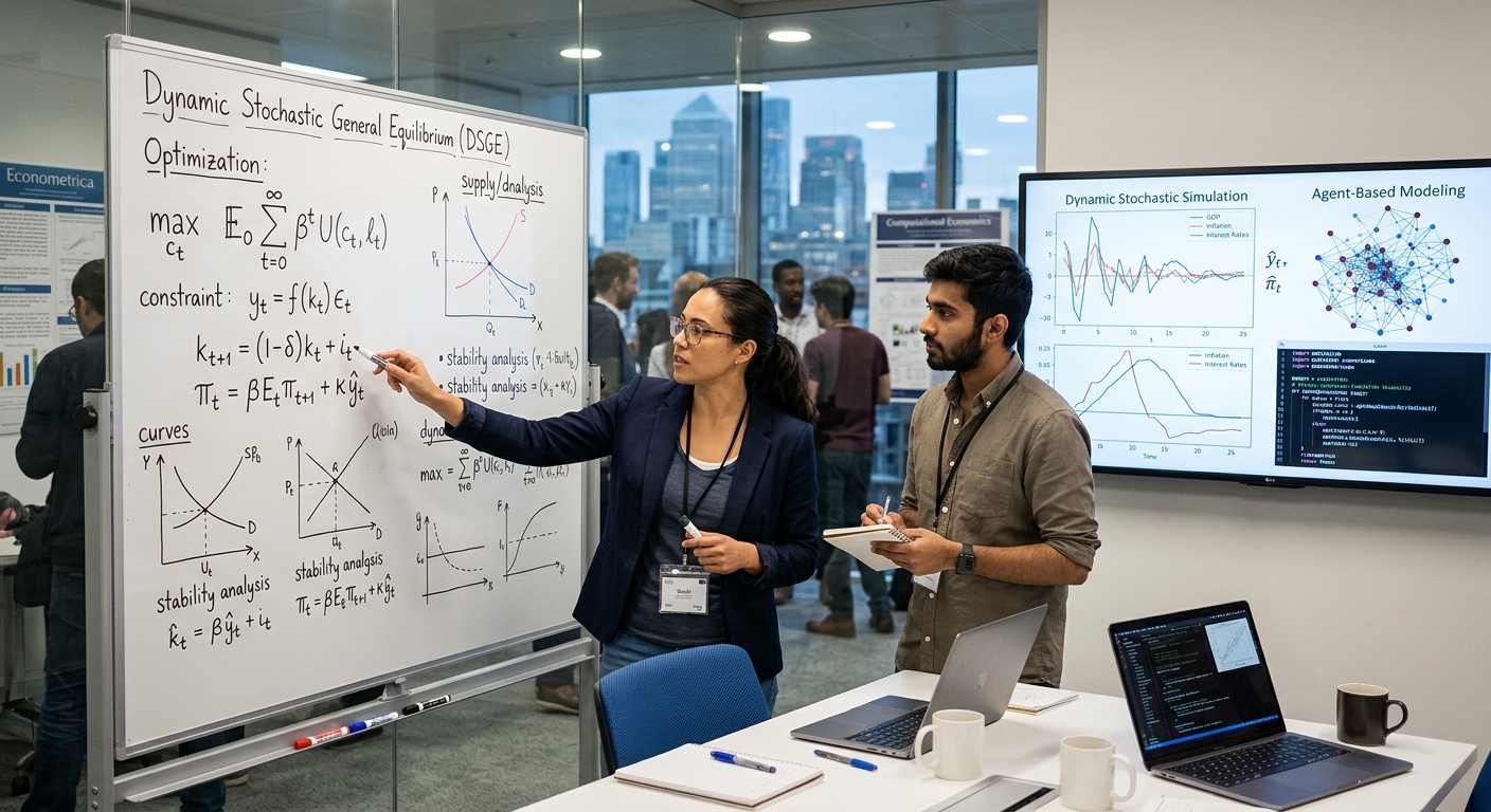
An interdisciplinary study of mathematics, economic theory, business intelligence, artificial intelligence, financial systems, and national development.
Abstract
Modern mathematical economics is the scientific study of how individuals, businesses, financial institutions, governments, and entire economies make decisions when resources are limited and human needs are numerous. It uses mathematical equations, statistical methods, optimisation techniques, probability theory, and computational models to understand economic behaviour and improve decision-making.
Mathematics enables economists to move beyond general statements such as prices rise when demand increases and investigate more precise questions:
- How much might demand change when a product’s price increases by 10%?
- How should a business allocate a limited budget among competing projects?
- What combination of labour, machinery, energy, and technology produces the greatest output?
- How can a government improve employment, productivity, infrastructure, and economic growth?
- How can artificial intelligence help predict demand, detect economic risks, and allocate resources more efficiently?
Mathematical economics is particularly important in a modern economy where data, computing power, automation, international trade, digital banking, and artificial intelligence increasingly influence production and consumption.
Central thesis: Mathematical economics provides a structured framework for understanding economic relationships, evaluating alternative decisions, and designing more efficient economic systems. Its greatest value comes from combining mathematical precision with reliable data, realistic assumptions, institutional knowledge, and human judgement.
Chapter 1. The foundations of mathematical economics
1.1 What is an economy?
An economy is a system through which society produces, distributes, exchanges, and consumes goods and services.
Every economy faces three fundamental questions:
- What should be produced? Food, housing, healthcare, computers, energy, transport, or other goods and services?
- How should it be produced? Through labour, machinery, technology, natural resources, or combinations of these?
- Who receives the output? How are goods, services, income, and opportunities distributed?
These questions arise because resources are limited. Even a technologically advanced country cannot produce everything immediately or without cost.
Mathematical economics represents these choices using variables, equations, constraints, and objective functions.
1.2 The principal mathematical components
Algebra and equations
Describe relationships between price, quantity, income, cost, output, and profit.
Calculus
Measures marginal changes and helps determine optimal prices, production levels, and investment allocations.
Statistics and econometrics
Use observed data to estimate relationships and test whether economic explanations are supported by evidence.
Optimisation and operations research
Identify the best feasible decision when budgets, time, labour, materials, or production capacity are limited.
Computational economics
Uses computers, simulation, numerical methods, and increasingly AI to investigate complex economic systems.
These branches complement one another. Algebra builds a model, calculus investigates how it changes, statistics tests it against data, optimisation identifies possible improvements, and computing allows more complex models to be evaluated.
Chapter 2. The basic mathematical language of economics
Economic models often begin by identifying the quantities that matter.
| Symbol | Economic meaning | Example |
|---|---|---|
| \(P\) | Price | Price per kilogram |
| \(Q\) | Quantity | Kilograms sold |
| \(Y\) | Income or output, depending on context | Household income |
| \(C\) | Cost or consumption, depending on context | Production cost |
| \(R\) | Revenue | Sales income |
| \(\pi\) | Profit | Revenue minus cost |
| \(L\) | Labour | Hours worked |
| \(K\) | Capital | Machinery, equipment, buildings |
| \(r\) | Interest rate or return, depending on context | Borrowing rate |
| \(g\) | Growth rate | Annual output growth |
The meaning of a symbol depends on the model. Economists therefore define variables before using equations.
2.1 Functions
A function describes how one quantity depends on another.
For example, a simple demand function is:
\[ Q_d=a-bP \]
Where:
- \(Q_d\) is the quantity consumers wish to buy.
- \(a\) represents the baseline level of demand.
- \(P\) is the price.
- \(b\) measures how strongly quantity demanded responds to price.
Suppose:
\[ Q_d=1{,}000-20P \]
At a price of 10 monetary units:
\[ Q_d=1{,}000-20(10)=800 \]
The model predicts demand of 800 units at that price.
At a price of 20:
\[ Q_d=1{,}000-20(20)=600 \]
Within this illustrative model, the higher price corresponds to a reduction of 200 units in quantity demanded.
This is not a universal prediction. Actual demand also depends on income, competition, preferences, product quality, and other factors.
2.2 Constraints
A constraint describes a limit on what is possible.
A business might have a budget of 100,000 monetary units. If \(x\) and \(y\) are quantities of two resources costing 200 and 500 units respectively, the budget constraint is:
\[ 200x+500y\leq100{,}000 \]
The inequality means that total expenditure must not exceed the available budget.
Constraints are essential because an economically attractive plan is not necessarily feasible.
Chapter 3. Supply, demand, and market equilibrium
Supply and demand are among the most important applications of mathematical economics.
- Demand represents how much consumers are willing and able to purchase at different prices.
- Supply represents how much producers are willing and able to sell at different prices.
- Market equilibrium occurs when the quantity supplied equals the quantity demanded, assuming the market can adjust to that point.
3.1 A mathematical equilibrium model
Suppose the demand and supply equations for a product are:
\[ Q_d=1{,}000-20P \]
\[ Q_s=100+10P \]
At equilibrium:
\[ Q_d=Q_s \]
Therefore:
\[ 1{,}000-20P=100+10P \]
Rearranging:
\[ 900=30P \]
\[ \boxed{P^*=30} \]
Substitute the equilibrium price into either equation:
\[ Q^*=1{,}000-20(30) \]
\[ \boxed{Q^*=400} \]
Illustrative market equilibrium
Equilibrium price
30
Monetary units per product
Equilibrium quantity
400
Units traded
These values are hypothetical and demonstrate the method, not an observed market.
The model helps a business or economist estimate the price and quantity at which planned purchases and planned sales match. Actual markets can differ because of taxes, price controls, imperfect competition, changing expectations, and other influences.
3.2 What happens when conditions change?
Consider a rise in consumer income that increases demand. At every given price, buyers now want more of the product.
If supply remains unchanged, the equilibrium price and quantity generally rise in this model.
By contrast, if a production innovation reduces costs and shifts supply outward, equilibrium quantity generally rises while equilibrium price falls.
This is why economic analysis must distinguish between a movement along a curve and a shift of the entire curve.
Chapter 4. Consumer behaviour and utility maximisation
Consumers have limited incomes but many competing needs. Mathematical economics investigates how they allocate their budgets.
4.1 The budget constraint
Suppose a household has 1,000 monetary units to spend on food and transport.
Let:
- \(F\) = units spent on food.
- \(T\) = units spent on transport.
- \(p_F\) and \(p_T\) = their respective prices.
The budget constraint is:
\[ p_FF+p_TT\leq1{,}000 \]
The household must choose an affordable combination.
However, affordability alone does not determine the decision. The household also considers the usefulness of each purchase.
4.2 The utility function
Economists represent consumer preferences using a utility function. One illustrative function is:
\[ U(F,T)=F^{0.5}T^{0.5} \]
The objective is to maximise \(U\), subject to the budget constraint.
The function represents a preference for having both goods rather than spending everything on only one, under the model’s assumptions.
More generally:
\[ \max_{F,T} U(F,T) \]
subject to:
\[ p_FF+p_TT\leq M \]
where \(M\) is household income.
This is a constrained optimisation problem.
4.3 Why this matters in the modern economy
Consumer optimisation models help economists investigate:
- How households respond to changes in food and electricity prices.
- How taxes affect purchasing decisions.
- How income changes influence consumption.
- How governments can evaluate the distributional effects of policies.
- How businesses can understand customer preferences without assuming that every customer behaves identically.
Real households also face uncertainty, credit constraints, habits, family obligations, and unequal access to information. A mathematical model should account for these factors when they materially affect the question.
Chapter 5. Production theory and business efficiency
Production theory investigates how businesses convert inputs into outputs.
Typical inputs include:
- Labour and skills.
- Machinery and equipment.
- Land and buildings.
- Electricity and fuel.
- Raw materials.
- Software, data, and intellectual property.
- Research and technological innovation.
A production function represents the relationship between inputs and output.
5.1 The Cobb–Douglas production function
A widely used example is:
\[ Y=AK^\alpha L^\beta \]
Where:
- \(Y\) = total output.
- \(A\) = productivity or technology factor.
- \(K\) = capital.
- \(L\) = labour.
- \(\alpha,\beta\) = parameters describing output responses to the inputs.
Suppose:
\[ Y=2K^{0.4}L^{0.6} \]
If capital is 100 units and labour is 100 units:
\[ Y=2(100)^{0.4}(100)^{0.6}=200 \]
The model predicts 200 units of output.
This example assumes the same production technology and consistent measurement units. It is not an empirical estimate for a real company.
5.2 Returns to scale
The sum \(\alpha+\beta\) determines the returns to scale for this production function.
| Condition | Interpretation |
|---|---|
| \(\alpha+\beta=1\) | Constant returns to scale |
| \(\alpha+\beta>1\) | Increasing returns to scale |
| \(\alpha+\beta<1\) | Decreasing returns to scale |
For the example, \(0.4+0.6=1\). If both capital and labour doubled, output would double, assuming the function continued to apply.
This does not mean every real factory can double its output simply by doubling its inputs. Space, management, supply chains, skills, energy availability, and technology may impose additional constraints.
5.3 Productivity and innovation
Productivity concerns how effectively resources generate output.
A company can improve productivity by:
- Training workers.
- Reducing waste.
- Improving machinery.
- Automating repetitive processes.
- Improving energy efficiency.
- Using data to plan inventory.
- Redesigning production workflows.
- Improving the quality of products and services.
Mathematical economics can help compare the cost of these interventions with their expected benefits.
For example, a new machine may raise output but also increase maintenance costs and electricity consumption. A complete model evaluates the total change in costs and benefits, not output alone.
Chapter 6. Profit maximisation and marginal analysis
A business must understand the relationship between revenue, cost, and profit.
The basic equation is:
\[ \pi(Q)=R(Q)-C(Q) \]
Where:
- \(\pi\) = profit.
- \(R(Q)\) = total revenue.
- \(C(Q)\) = total cost.
- \(Q\) = output.
Consider this hypothetical business:
\[ R(Q)=100Q \]
\[ C(Q)=1{,}000+20Q+Q^2 \]
Therefore:
\[ \pi(Q)=80Q-Q^2-1{,}000 \]
The marginal profit condition for an interior optimum is:
\[ \frac{d\pi}{dQ}=0 \]
Differentiating gives:
\[ 80-2Q=0 \]
Thus:
\[ \boxed{Q^*=40} \]
The second derivative is:
\[ \frac{d^2\pi}{dQ^2}=-2 \]
Because it is negative, the profit function is concave, and this stationary point is a maximum.
Profit at this output is:
\[ \pi(40)=80(40)-40^2-1{,}000 \]
\[ \boxed{\pi(40)=600} \]
The result assumes the stated revenue and cost functions apply, output is continuously adjustable, and there are no additional constraints. All amounts are illustrative monetary units.
6.1 The marginal principle
The marginal cost is the additional cost of producing a little more output. Marginal revenue is the additional revenue generated by that output.
For an interior profit maximum under standard differentiability assumptions:
\[ \boxed{MR=MC} \]
This does not mean that every business should mechanically produce until these quantities match. Capacity limits, competition, uncertain demand, environmental costs, and other constraints can change the appropriate decision.
The principle is useful because it encourages managers to compare the additional benefit of an action with its additional cost.
Chapter 7. Calculus, marginal changes, and economic sensitivity
Calculus gives economists a method for studying how one variable changes when another variable changes.
7.1 First derivatives
Suppose a firm’s total cost is:
\[ C(Q)=500+10Q+0.5Q^2 \]
The marginal cost is the derivative:
\[ MC=\frac{dC}{dQ}=10+Q \]
At output \(Q=20\):
\[ MC=10+20=30 \]
The marginal cost at that output is 30 monetary units per additional unit, interpreted locally under the continuous model.
7.2 Second derivatives
A second derivative measures how the rate of change itself changes.
In economics, it can help determine whether marginal costs are rising or falling, whether a maximum or minimum has been found, and how curvature affects a decision.
For the cost function above:
\[ \frac{d^2C}{dQ^2}=1 \]
Since the second derivative is positive, marginal cost increases with output.
This may represent a factory that must use less efficient equipment, pay overtime, or work around capacity limitations as production expands.
7.3 Elasticity
Elasticity measures percentage responsiveness rather than absolute change.
Price elasticity of demand is:
\[ E_d=\frac{dQ}{dP}\frac{P}{Q} \]
For the demand function:
\[ Q=1{,}000-20P \]
the derivative is:
\[ \frac{dQ}{dP}=-20 \]
At \(P=20\), quantity is 600, so:
\[ E_d=-20\left(\frac{20}{600}\right) \]
\[ \boxed{E_d\approx-0.67} \]
The negative sign indicates that quantity demanded moves in the opposite direction to price in this model. The absolute value, about 0.67, indicates relatively inelastic demand at that point.
Elasticity matters because a 10% price increase does not necessarily cause a 10% change in sales. The response depends on the product, customer alternatives, time horizon, and market conditions.
Chapter 8. Linear algebra and the interdependence of industries
Modern economies consist of interconnected industries. Agriculture depends on fertiliser, transport, energy, finance, machinery, and communication. Manufacturing depends on raw materials, electricity, logistics, and business services.
Linear algebra helps represent these connections.
8.1 Input-output economics
An input-output model describes how much of each industry’s output is required to produce the output of other industries.
A standard simplified model is:
\[ \mathbf{x}=A\mathbf{x}+\mathbf{d} \]
Where:
- \(\mathbf{x}\) is the vector of total industry outputs.
- \(A\) is the matrix of intermediate input requirements.
- \(\mathbf{d}\) is final demand, such as household consumption or exports.
Rearranging:
\[ (I-A)\mathbf{x}=\mathbf{d} \]
If the inverse exists:
\[ \boxed{\mathbf{x}=(I-A)^{-1}\mathbf{d}} \]
This equation calculates the total production required to meet final demand, including intermediate inputs used throughout the economy.
8.2 A simple two-sector example
Imagine an economy with agriculture and manufacturing.
Suppose each unit of agricultural output requires 0.2 units of agricultural inputs and 0.1 units of manufactured inputs. Each unit of manufacturing requires 0.3 units of agricultural inputs and 0.2 units of manufactured inputs.
The input matrix is:
\[ A= \begin{bmatrix} 0.2&0.3\\ 0.1&0.2 \end{bmatrix} \]
Suppose final demand is:
\[ \mathbf{d}= \begin{bmatrix} 100\\ 80 \end{bmatrix} \]
The economy must produce more than the final demand quantities because industries also supply inputs to one another.
Solving the system gives approximately:
\[ \mathbf{x}= \begin{bmatrix} 164.62\\ 126.15 \end{bmatrix} \]
Thus, the model estimates total agricultural output of about 164.62 units and manufacturing output of about 126.15 units.
These figures are hypothetical. Real input-output tables require measured industry data, consistent units, and appropriate treatment of imports and taxes.
8.3 Strategic economic importance
Input-output analysis can help governments and businesses examine:
- How electricity shortages affect manufacturing and services.
- How transport disruptions influence food prices.
- How local suppliers contribute to industrial development.
- Which industries are heavily dependent on imports.
- How an increase in public infrastructure spending may affect demand across sectors.
The key insight is that an industry cannot always be analysed in isolation. A constraint in one sector can affect many others.
Chapter 9. Macroeconomic modelling: GDP, inflation, employment, and growth
Microeconomics studies individual consumers, firms, and markets. Macroeconomics studies the economy as a whole.
Mathematical macroeconomics investigates the relationships between national output, consumption, investment, employment, inflation, interest rates, government expenditure, and international trade.
9.1 Gross domestic product
The expenditure approach to GDP is:
\[ \boxed{Y=C+I+G+(X-M)} \]
Where:
- \(Y\) = gross domestic product.
- \(C\) = household consumption.
- \(I\) = investment in produced capital.
- \(G\) = government purchases of goods and services.
- \(X\) = exports.
- \(M\) = imports.
Suppose an economy records the following values, all in billions of monetary units:
| Component | Value |
|---|---|
| Consumption | 600 |
| Investment | 180 |
| Government purchases | 200 |
| Exports | 150 |
| Imports | 130 |
Then:
\[ Y=600+180+200+(150-130) \]
\[ \boxed{Y=1{,}000\text{ billion}} \]
This is a simplified illustration. Official GDP estimates require national accounting procedures, and real GDP must be distinguished from nominal GDP.
9.2 Nominal and real GDP
Nominal GDP measures output using prices of the period being measured. Real GDP adjusts for price changes to estimate changes in the volume of production.
This distinction matters because a rise in the monetary value of output does not necessarily mean that an economy is producing more goods and services.
9.3 Economic growth
A simple growth-rate formula is:
\[ g=\frac{Y_t-Y_{t-1}}{Y_{t-1}}\times100\% \]
Suppose real GDP increases from 1,000 billion to 1,050 billion.
\[ g=\frac{1{,}050-1{,}000}{1{,}000}\times100\% \]
\[ \boxed{g=5\%} \]
Real GDP growth is important, but it does not by itself measure income distribution, environmental sustainability, public health, or overall quality of life.
9.4 The aggregate production function
Long-run growth models often use:
\[ Y=AK^\alpha L^{1-\alpha} \]
Here, productivity \(A\), capital \(K\), and labour \(L\) contribute to aggregate output.
A country may improve long-term productive capacity through better infrastructure, education, health, technology, research, institutional quality, and effective competition.
Capital accumulation alone is not enough. Its productivity depends on how well the capital is maintained, managed, and used.
Chapter 10. Mathematical economics and monetary policy
Central banks analyse economic conditions when making decisions about interest rates and financial stability.
Mathematical models can help investigate relationships among:
- Inflation and inflation expectations.
- Interest rates and borrowing costs.
- Household consumption.
- Business investment.
- Exchange rates.
- Employment and economic output.
- Financial-sector risk.
10.1 A simplified interest-rate relationship
A commonly used conceptual relationship is:
\[ i\approx r+\pi^e \]
Where:
- \(i\) = nominal interest rate.
- \(r\) = real interest rate.
- \(\pi^e\) = expected inflation.
This is an approximation related to the Fisher equation. The exact relationship, under the standard formulation, is:
\[ 1+i=(1+r)(1+\pi^e) \]
Expected inflation matters because lenders and borrowers care about purchasing power, not merely the number of currency units exchanged.
10.2 Why interest rates influence economic activity
When interest rates rise, borrowing may become more expensive. Some households may delay major purchases, and some businesses may postpone investment.
Higher rates can also affect savings returns, currency demand, asset prices, and expectations. The actual effects depend on economic conditions and may occur with delays.
Mathematical models help policymakers estimate these relationships, but they cannot eliminate uncertainty or guarantee a particular outcome.
Chapter 11. Econometrics: testing economic theories against evidence
Mathematical economics builds formal models. Econometrics uses statistical methods to estimate and evaluate relationships using data.
An equation can be mathematically correct while its assumptions are unrealistic. Econometric analysis helps assess whether the proposed relationships are supported by observed evidence.
11.1 Regression analysis
A basic linear regression model is:
\[ Y_i=\beta_0+\beta_1X_i+\varepsilon_i \]
Where:
- \(Y_i\) is the outcome being studied.
- \(X_i\) is an explanatory variable.
- \(\beta_0\) is the intercept.
- \(\beta_1\) is the estimated relationship.
- \(\varepsilon_i\) represents factors not captured by the model.
For example, a researcher might investigate the relationship between years of education and earnings.
If the estimated coefficient on education is positive, the data show a positive conditional association within the model. That result alone does not prove that additional education caused the earnings difference. Family circumstances, prior ability, job opportunities, and other factors may influence both.
11.2 Correlation versus causation
Suppose sales increase at the same time as advertising expenditure increases.
There are several possible explanations:
- Advertising increased sales.
- The business advertised because it expected sales to increase.
- A seasonal event raised both advertising and sales.
- A price change or competitor’s decision affected both variables.
To investigate causation, researchers may use randomised experiments where feasible, natural experiments, instrumental variables, difference-in-differences methods, or other credible research designs.
The choice depends on the question and the quality of the available data.
11.3 Forecasting and uncertainty
Economic forecasting uses historical data, current indicators, and model assumptions to estimate future conditions.
Forecasts should include uncertainty because future prices, demand, employment, production, and policy conditions may differ from expectations.
A responsible economic forecast is a conditional estimate, not a promise.
Chapter 12. Game theory, competition, and strategic decision-making
Game theory is the mathematical study of situations in which one person’s or organisation’s best decision depends on the decisions of others. It is used to analyse competition, bargaining, auctions, cooperation, voting, and market strategy. MIT OpenCourseWare
12.1 The basic structure of a game
A mathematical game typically contains:
- Players: The people, businesses, or institutions making decisions.
- Strategies: The actions available to each player.
- Payoffs: The benefits or costs associated with the resulting outcomes.
- Information: What each player knows when making a decision.
- Rules: The conditions under which decisions are made.
12.2 A simple business example
Two companies must choose whether to invest in product innovation.
| Company B: Low investment | Company B: High investment | |
|---|---|---|
| Company A: Low investment | (5, 5) | (2, 7) |
| Company A: High investment | (7, 2) | (6, 6) |
Illustrative payoffs in arbitrary units. Each pair is (Company A, Company B).
This table demonstrates that the best decision for one company depends partly on what the other company does.
Game theory can help businesses analyse competitive pricing, research investment, negotiations, platform competition, and cooperation between suppliers.
However, a mathematical prediction depends on the assumed payoffs, available strategies, and information. Real companies may behave differently because of uncertainty, reputation, regulation, and long-term relationships.
Chapter 13. Mathematical optimisation and resource allocation
Optimisation is one of the most practical branches of mathematical economics. It helps identify the best feasible decision according to a specified objective.
Economists may seek to maximise:
- Business profit.
- Agricultural output.
- Economic productivity.
- Social welfare.
- Infrastructure benefits.
- Energy efficiency.
They may also seek to minimise costs, delays, pollution, or resource waste.
13.1 Linear programming
Consider a small agricultural business producing two products: crop A and crop B.
Let:
- \(x\) = units of crop A.
- \(y\) = units of crop B.
Suppose contribution to profit is 40 units per unit of crop A and 30 units per unit of crop B.
The objective is:
\[ \max Z=40x+30y \]
The available resources impose these constraints:
\[ 2x+y\leq100 \]
\[ x+2y\leq80 \]
\[ x,y\geq0 \]
The first constraint represents one limited resource, while the second represents another. The exact interpretation could be land, labour, water, or machine hours.
To investigate a corner where both resource constraints bind, solve:
\[ 2x+y=100 \]
\[ x+2y=80 \]
From the first equation:
\[ y=100-2x \]
Substituting into the second:
\[ x+2(100-2x)=80 \]
\[ -3x=-120 \]
\[ x=40,\qquad y=20 \]
The objective value is:
\[ Z=40(40)+30(20)=2{,}200 \]
Checking the other feasible corner points shows that this solution gives the highest objective value for this particular model.
Optimisation result
40
Units of crop A
20
Units of crop B
Maximum objective value
2,200
This is a hypothetical result. It assumes divisible production quantities and the stated resource and contribution values.
Linear programming is useful in farming, manufacturing, logistics, transport planning, staffing, and energy distribution. Its limitations include uncertainty, inaccurate input estimates, and objectives that cannot easily be expressed in monetary units.
Chapter 14. Dynamic economics: decisions over time
Many economic decisions involve a sequence of choices rather than a single decision.
A business invests today to produce goods in the future. A government builds infrastructure that may deliver benefits for decades. A household saves income to meet future needs.
Dynamic economic models represent how decisions and economic variables evolve over time.
14.1 Compound growth
A basic discrete-time growth equation is:
\[ K_{t+1}=(1-\delta)K_t+I_t \]
Where:
- \(K_t\) = capital stock at time \(t\).
- \(\delta\) = depreciation rate.
- \(I_t\) = investment during the period.
The equation states that next period’s capital equals the capital that remains after depreciation plus new investment.
If capital is 1,000 units, depreciation is 5%, and investment is 100 units:
\[ K_{t+1}=0.95(1{,}000)+100 \]
\[ \boxed{K_{t+1}=1{,}050} \]
The model helps explain why an economy must invest not only to expand capacity but also to replace worn-out equipment and infrastructure.
14.2 Discounting future benefits
Future costs and benefits are often expressed in present-value terms:
\[ PV=\frac{FV}{(1+r)^n} \]
Where:
- \(PV\) = present value.
- \(FV\) = future monetary value.
- \(r\) = discount rate per period.
- \(n\) = number of periods.
If a project is expected to generate 121 monetary units two years from now and the annual discount rate is 10%:
\[ PV=\frac{121}{(1.10)^2}=100 \]
Its future benefit has a present value of 100 under these assumptions.
For a real investment, decision-makers should also consider risk, maintenance, taxes, inflation, environmental effects, and benefits that cannot be fully represented by monetary values.
Chapter 15. Mathematical economics in artificial intelligence and digital systems
Modern computational economics combines mathematical models, large datasets, algorithms, and computing systems.
Artificial intelligence can support economic analysis, but it does not replace the need for sound economic reasoning.
AI Boom Balances Headwinds: Macroeconomics Outlook 2026 – AI CERTs News
1. Economic forecasting
Statistical and machine-learning models can analyse historical demand, prices, output, and other indicators to estimate future conditions.
2. Intelligent production planning
Algorithms can help schedule machines, estimate inventory needs, coordinate supply chains, and reduce production waste.
Smart Crop Monitoring Market Expected to Reach US$ 10.30 Billion
3. Agricultural economics
Data models can support crop planning, resource allocation, yield estimation, and analysis of input costs and market demand.
Isometric Global Digital Finance Network with Online Banking
4. Digital finance
Mathematical and statistical models can help evaluate credit risk, forecast cash flows, detect unusual transactions, and measure financial exposure.
15.1 An AI-supported economic decision system
A responsible system can be organised as follows:
Economic data
Prices, costs, output, employment, demand
Mathematical model
Equations, constraints, statistical relationships
AI and computational analysis
Forecasts, simulations, alternative scenarios
Human evaluation
Check assumptions, fairness, risks, and feasibility
Decision and monitoring
Implement, measure outcomes, revise the model
This structure is important because AI can detect patterns that are not causal, reproduce biases in historical data, or produce inaccurate predictions when economic conditions change.
The final decision should therefore be supported by evidence, appropriate safeguards, and ongoing evaluation.
Chapter 16. Mathematical economics and national development in South Africa
Mathematical economics can support development planning by helping institutions compare resource needs, costs, expected outcomes, and competing priorities.
For South Africa, relevant areas include electricity supply, logistics, agriculture, manufacturing, digital infrastructure, education, employment, and small-business productivity.
The following are applications of the methods discussed above, not claims that a particular policy has already achieved the stated results.
16.1 Agricultural development
A farm’s production plan can be modelled using:
\[ \max \pi = \text{Revenue} – \text{Production costs} \]
Subject to constraints on land, water, labour, energy, equipment, and available capital.
A more complete model might include uncertain crop yields, seasonal prices, soil conditions, irrigation requirements, and transportation costs.
This can help compare alternative production plans and identify which resource constraints most limit the business.
16.2 Electricity and infrastructure
Infrastructure planning involves balancing capital expenditure, operating costs, capacity, reliability, and future demand.
Optimisation can help compare where additional capacity or maintenance may provide the greatest benefit, subject to engineering and regulatory constraints.
Economic models should also account for the wider effects of unreliable electricity on factories, farms, hospitals, schools, and digital services.
16.3 Employment and skills
A government or institution may compare the costs and expected benefits of vocational training, apprenticeships, digital education, and technical qualifications.
Evaluation should distinguish between participation in a programme and its actual effect on employment, productivity, wages, and business creation.
Reliable comparisons require evidence about what would likely have happened without the intervention.
16.4 Industrial policy and local supply chains
Input-output analysis can help identify how local manufacturing, agriculture, logistics, and business services depend on one another.
It can also help estimate the domestic production required to meet changes in final demand, subject to the assumptions of the model.
However, local production is not automatically more efficient in every case. Decisions should consider productivity, quality, scale, competition, technology, and long-term economic resilience.
Chapter 17. Welfare economics, inequality, and social priorities
Economic efficiency and social welfare are related but distinct concepts.
An allocation can maximise total output or total surplus without distributing the benefits fairly. Mathematical economics therefore studies not only what can be produced, but also how economic outcomes affect different groups.
17.1 Social welfare functions
A simplified social welfare function might be:
\[ W=W(U_1,U_2,\ldots,U_n) \]
Where \(U_i\) represents the welfare or utility of person \(i\).
Different social welfare functions assign different weights to individual outcomes. A policy that increases total income might have different implications depending on whether the gains are widely shared or concentrated among a small group.
17.2 Externalities
An externality occurs when an activity affects people who are not fully represented in the market transaction.
Examples include:
- Air pollution from industrial production.
- Noise from transport.
- Knowledge spillovers from scientific research.
- Public-health benefits from disease prevention.
Suppose a factory’s private marginal cost is \(MC_p\), but pollution imposes an additional marginal cost on society, \(MEC\).
Then:
\[ MSC=MC_p+MEC \]
Where \(MSC\) is marginal social cost.
A market decision based only on private cost may produce more pollution than is socially desirable. Environmental standards, taxes, tradable permits, or other policies may help address the difference, depending on circumstances and implementation.
17.3 The limits of monetary measurement
Not every important social outcome can be reduced to a single monetary number. Human dignity, equal treatment, environmental protection, public safety, and access to essential services may require separate indicators and explicit ethical choices.
A good mathematical model makes its objectives visible rather than hiding value judgements inside equations.
Chapter 18. The limitations and risks of mathematical economic models
Mathematical economics is powerful, but a model is a simplified representation of reality.
Its reliability depends on the quality of its assumptions, data, structure, and interpretation.
| Limitation | Why it matters | Appropriate response |
|---|---|---|
| Incomplete data | Important economic relationships may be missed | Improve data quality and disclose gaps |
| Incorrect assumptions | Predictions may not reflect actual behaviour | Test alternative assumptions |
| Changing conditions | Historical patterns may no longer hold | Re-estimate and monitor models |
| Human behaviour | People may not behave as the model predicts | Incorporate behavioural evidence |
| Distributional effects | Average gains can conceal losses for some groups | Report outcomes across different groups |
| Model uncertainty | Several models may produce different results | Compare models and show uncertainty |
| Ethical concerns | Efficiency may conflict with fairness or other goals | Make objectives and trade-offs explicit |
18.1 The danger of false precision
A model may produce a result such as 17.4382%, but that many decimal places do not make the estimate accurate.
When input data are uncertain, assumptions are simplified, and future behaviour is unpredictable, results should be reported at a precision appropriate to the evidence.
18.2 Mathematical correctness versus economic usefulness
Three questions should always be separated:
- Is the mathematics correct?
- Does the model adequately represent the economic situation?
- Is the decision desirable after considering wider social, ethical, and practical consequences?
A model can answer the first question correctly while failing the second or third.
Chapter 19. A practical framework for solving economic problems
The following framework can be used by students, entrepreneurs, researchers, and development planners.
- Define the economic problem. State the decision, objective, affected groups, and relevant time period.
- Collect reliable data. Identify prices, quantities, costs, income, capacity, and other relevant variables.
- Build the mathematical model. Choose suitable equations, functions, constraints, and assumptions.
- Solve the problem. Use algebra, calculus, statistics, optimisation, or computational techniques as appropriate.
- Test the model. Check the calculations, compare predictions with observations, and examine alternative assumptions.
- Compare scenarios. Consider changes in demand, costs, technology, interest rates, or available resources.
- Evaluate consequences. Examine feasibility, uncertainty, distributional effects, and environmental implications.
- Implement and monitor. Compare actual outcomes with expected outcomes and revise the model when necessary.
The objective is not simply to obtain an answer from an equation. It is to improve the quality of the decision.
Chapter 20. Future directions of mathematical economics
Several important developments are shaping the field.
Computational macroeconomics: Researchers use numerical methods and simulations to investigate how households, businesses, financial markets, and governments interact over time.
Network economics: Mathematical networks help explain how shocks spread through supply chains, banking systems, communication systems, and international trade.
Behavioural economics: Models increasingly incorporate evidence that human decisions may be influenced by habits, limited attention, imperfect information, and social preferences.
Environmental economics: Mathematical methods support the analysis of resource scarcity, energy transitions, pollution, climate risks, and the economic consequences of environmental policies.
Digital and AI economics: Researchers study digital platforms, automated production, data as an economic asset, algorithmic decision-making, and how AI may change productivity and labour demand.
Uncertainty and resilience: Stochastic models, scenario analysis, and robust optimisation help decision-makers examine a range of possible futures instead of relying on one forecast.
These directions extend established mathematical methods rather than making them obsolete. The central tasks remain defining the problem, selecting an appropriate model, evaluating evidence, and understanding the limits of the conclusions.
Chapter 21. Essential mathematical formulas: a revision guide
| Economic concept | Formula | Main purpose |
|---|---|---|
| Revenue | \(R=PQ\) | Calculate sales income at a uniform price |
| Profit | \(\pi=R-C\) | Calculate revenue less total cost |
| Market equilibrium | \(Q_d=Q_s\) | Find the price and quantity at which demand equals supply |
| Price elasticity | \(E_d=\frac{dQ}{dP}\frac{P}{Q}\) | Measure demand responsiveness |
| Marginal cost | \(MC=\frac{dC}{dQ}\) | Measure the additional cost of output |
| Profit maximisation | \(MR=MC\) | Identify an interior optimum under standard assumptions |
| GDP expenditure | \(Y=C+I+G+(X-M)\) | Calculate GDP using the expenditure approach |
| Growth rate | \(g=\frac{Y_t-Y_{t-1}}{Y_{t-1}}\times100\%\) | Measure percentage growth |
| Present value | \(PV=\frac{FV}{(1+r)^n}\) | Convert a future monetary value into present-value terms |
| Production | \(Y=AK^\alpha L^\beta\) | Model output from capital, labour, and productivity |
| Input-output model | \(\mathbf{x}=(I-A)^{-1}\mathbf{d}\) | Estimate total production needed for final demand |
These formulas represent different economic relationships. They are not interchangeable, and each requires suitable assumptions and definitions.
Conclusion
Modern mathematical economics provides a rigorous way to investigate how scarce resources can be allocated, how markets operate, how businesses make decisions, and how economies develop over time.
Its foundation combines mathematical reasoning with economic theory. Algebra explains relationships, calculus measures marginal changes, optimisation identifies feasible choices, linear algebra represents interconnected industries, statistics tests hypotheses, and computational methods allow more complex systems to be investigated.
Its applications extend from the price of a single agricultural product to national infrastructure, financial stability, industrial policy, digital technology, and global economic networks.
The most important principle is that mathematics improves economic reasoning when it is used to clarify assumptions, test evidence, compare alternatives, and recognise uncertainty. It does not remove the need for sound judgement or guarantee that an economically efficient decision will automatically be fair, sustainable, or socially desirable.
For South Africa and other developing and industrial economies, the opportunity is to combine mathematical literacy, scientific research, quality data, technological innovation, and capable institutions to make better-informed economic decisions.
Recommended academic reading and learning resources
The following resources provide a foundation for studying the methods developed in this thesis.
Mathematical Economics: Prelude to the Neoclassical Model | Springer Nature Link
1. Mathematical Economics: Prelude to the Neoclassical Model — Kam Yu.
Covers mathematical foundations, linear algebra, optimisation, probability, and dynamic modelling.
Quantitative methods for economics
2. Mathematics for Economists — Katherine Eyal, University of Cape Town.
A useful South African university resource covering optimisation, linear algebra, comparative statics, and differential equations.
Introduction to optimization for economists | Open Press Tilburg University
3. Introduction to Optimization for Economists — Jacob Engwerda.
An accessible introduction to constrained optimisation, linear programming, and decisions involving multiple objectives.
Lecture 22: Signaling | Economic Applications of Game Theory | Economics | MIT OpenCourseWare
4. Economic Applications of Game Theory — MIT OpenCourseWare.
Course materials on strategic interaction, competition, bargaining, and mathematical game theory.
For a logical learning sequence, start with algebra and functions, proceed to calculus and linear algebra, study microeconomics and macroeconomics, and then develop skills in econometrics, optimisation, and computational economics. This progression is consistent with the mathematical preparation outlined in the University of Cape Town and Springer resources. open.uct.ac.za






Be First to Comment